
Introduction to spreadsheets (Microsoft excel) and Data Validation

A spreadsheet program is a software that help you manage analyze and present data the way you like. Spreadsheet programs can quickly carry out several important functions on data. A spreadsheet consists of a grids made from columns and rows.
What is Microsoft Excel?
Microsoft Excel is a Spreadsheet Application Software which is run by Windows Operating System, which is used for analyzing arithmetical calculations and presenting data in various forms, e.g. numeric values, character, string etc., is one of the Microsoft Office packages.
Microsoft Excel is commonly used in:
- Accounting natured jobs
- Statistical nature jobs and
- Mathematical analysis
Microsoft excel screen or windows features
Workbook is a set of worksheets store in a single file. Workbooks are convenient for organizing related spreadsheets into the same file, you could keep the sales data for each quarter on a separate worksheet within a single workbook
Worksheet is a basic spreadsheet made from columns and rows in which you can enter data. It’s a single page in the workbook
Columns are vertical lines drawn from top to bottom of the worksheet. They are labeled with letters. The first letter is A and the last is IV, they are labeled from left to right at the top of the worksheet . The total number of columns is 256.
Rows are horizontal lines drawn from left to right of the worksheet. They are labeled with numbers from top to bottom. There are 65,536 rows in a single worksheet
Cell is an intersection between column and row e.g. A1 is an intersection between column A and row 1.
Active Cell the cell affected by the actions you do, is enclosed with a thick border.
Cell pointer indicates the Active Cell.
Mouse pointer indicates the position of a mouse arrow, it change its appearance depending on the position it points.
Cell Reference is a cell address that tell excel to perform operations using the data currently in the designated cells. Is the way of naming excel cells
Fill Handle
Is the dot at the bottom right of the active cell if you hold down your mouse on it and drag it excel will copy the cell data or formula to a cell you select while dragging.
Is an excel trick for spreading up data series for example if you are creating labels for months of the year ,you don’t have to type each month individually. In this case you just have to enter the first two numbers in the series ,excel uses the interval between these two numbers to determine which numbers should follow.
Dragging
Point to an item hold the mouse button down and move the mouse so that the object you pointed follow.
How to move through the worksheet
CTRL + Home - Moves you to the beginning of the worksheet
CTRL + End - Moves you to the end of the typed area
Working with multiple Sheets;
You can organize your work by keeping related information in separates worksheets within the same file (workbook)
You can insert work sheet just as you can insert additional rows and column.
> Inserting a new worksheet.
> Steps
> Click on insert menu
> Select worksheet
Moving a Worksheet
To move a Worksheet to different location, do the following: -
> Click on the tab of the sheet to be moved e.g. sheet four
> Drag the selected tab to new location
> Naming worksheet
> Double click on the worksheet tab e.g. Sheet1
> Enter a new name
> Press enter
> Copying a worksheet
To copy a worksheet to a different location, do the following:-
> Click on the tab representing the sheet to be copied
> While holding down the Ctrl key drag the selected Tab (sheet) to a new location
Deleting a worksheet.
> Steps
> Right click on the worksheet to be deleted
> Select delete from the pop up menu
How to Insert a Column or Row
> Position the mouse pointer to the cell next to the one you want to insert a column or row
> Click on insert Menu
> Select column or row
Or do one of the following:
> To insert a single row, select the row or a cell in the row above which you want to insert the new row. For example, to insert a new row above row 5, click a cell in row 5.
> To insert multiple rows, select the rows above which you want to insert rows. Select the same number of rows as you want to insert. For example, to insert three new rows, you need to select three rows.
> To insert nonadjacent rows, hold down CTRL while you select nonadjacent rows.
How to select cells, ranges, rows, or columns
> To select Do this A single cell Click the cell, or press the arrow keys to move to the cell. A range of cells Click the first cell in the range, and then drag to the last cell, or hold down SHIFT while you press the arrow keys to extend the selection. You can also select the first cell in the range, and then press F8 to extend the selection by using the arrow keys. To stop extending the selection, press F8 again.
A large range of cells Click the first cell in the range, and then hold down SHIFT while you click the last cell in the range. You can scroll to make the last cell visible. All cells on a worksheet Click the Select All button.
To select the entire worksheet, you can also press CTRL+A.
Note: If the worksheet contains data, CTRL+A selects the current region. Pressing CTRL+A a second time selects the entire worksheet.
Nonadjacent cells or cell ranges Select the first cell or range of cells, and then hold down CTRL while you select the other cells or ranges. You can also select the first cell or range of cells, and then press SHIFT+F8 to add another nonadjacent cell or range to the selection. To stop adding cells or ranges to the selection, press SHIFT+F8 again.
Note: You cannot cancel the selection of a cell or range of cells in a nonadjacent selection without canceling the entire selection.
An entire row or column Click the row or column heading.
Row heading
Column heading
You can also select cells in a row or column by selecting the first cell and then pressing CTRL+SHIFT+ARROW key (RIGHT ARROW or LEFT ARROW for rows, UP ARROW or DOWN ARROW for columns).
Note: If the row or column contains data, CTRL+SHIFT+ARROW key selects the row or column to the last used cell. Pressing CTRL+SHIFT+ARROW key a second time selects the entire row or column.
Adjacent rows or columns Drag across the row or column headings. Or select the first row or column; then hold down SHIFT while you select the last row or column. Nonadjacent rows or columns Click the column or row heading of the first row or column in your selection; then hold down CTRL while you click the column or row headings of other rows or columns that you want to add to the selection. The first or last cell in a row or column Select a cell in the row or column, and then press CTRL+ARROW key (RIGHT ARROW or LEFT ARROW for rows, UP ARROW or DOWN ARROW for columns). The first or last cell on a worksheet or in a Microsoft Office Excel table Press CTRL+HOME to select the first cell on the worksheet or in an Excel list. Press CTRL+END to select the last cell on the worksheet or in an Excel list that contains data or formatting.
Cells to the last used cell on the worksheet (lower-right corner) Select the first cell, and then press CTRL+SHIFT+END to extend the selection of cells to the last used cell on the worksheet (lower-right corner). Cells to the beginning of the worksheet Select the first cell, and then press CTRL+SHIFT+HOME to extend the selection of cells to the beginning of the worksheet. More or fewer cells than the active selection Hold down SHIFT while you click the last cell that you want to include in the new selection. The rectangular range between the active cell (active cell: The selected cell in which data is entered when you begin typing. Only one cell is active at a time. The active cell is bounded by a heavy border.) and the cell that you click becomes the new selection. Tip To cancel a selection of cells, click any cell on the worksheet.
On the Home tab, in the Cells group, click the arrow next to Insert, and then click Insert Sheet Rows.
Tip: You can also right-click the selected rows and then click Insert on the shortcut menu.
Note: When you insert rows on your worksheet, all references that are affected by the insertion adjust accordingly, whether they are relative (relative reference: In a formula, the address of a cell based on the relative position of the cell that contains the formula and the cell referred to. If you copy the formula, the reference automatically adjusts. A relative reference takes the form A1.) or absolute references. The same applies to deleting rows, except when a deleted cell is directly referenced by a formula. If you want references to adjust automatically, it's a good idea to use range references whenever appropriate in your formulas, rather than specifying individual cells.
Deleting Row or Column
You may find yourself needing to delete a row or column
Steps
Select the row or column to be deleted (to select the column to be deleted using the keyboard, press Ctrl + space bar, to select the row to be deleted using the key board, press shift + space bar)
Click on edit menu
Select delete
Applying or Setting Borders
Highlight your data
Click on format menu
Select cells
Select border tab
*Under presets
Select inside or outline
Select border style by selecting the style and then click inside your borders
Click on color, pick the color you want and click on your borders in order to change the color
Click ok
Formatting numbers
When entering values, excel automatically uses the format which omits decimal places, Excel however, allows you to access other built- in format (such as percentage signs, dollar signs, etc.).
Steps
Select the cells to format
Click on the format menu
Select cells
Click on the number tab
Select e.g. Number, Currency, and Percentage
Click ok.
Adjusting Column Width:
*You can change the Width of column by: -
Clicking on format menu and select column width OR
Dragging the column border inside the column heading OR
By double clicking the right column border (this is the best fit method)
Changing Row Height
*You can change row height by: -
Clicking on format menu, then select row height OR
Dragging the bottom row border at the row heading.
Merging cells
Select the cell to merge (merge them before entering data)
Click on format menu
Click cells
Select alignment tab
Activate merge cell
Click Ok
Formulas and functions
In electronic spreadsheets cells don’t have to contain fixed data rather they can contain formulas, which are set of instructions that perform calculations and display results. formula can be as simple as =2+2.But it is useful to use cell reference, the formula results change automatically. Any formula in spreadsheets begins with = sign
Operators
An operator is a special symbol that tells a program what action to take on a series of numbers.
There are mainly two types of operators
1. Mathematical operators
2. Logical operators
Mathematical operators
All computer programs use a common set of symbols to represent the four mathematical operators. These are four basic mathematical Operators

Whenever you want to use a formula in the cell make sure your formula starts with an equal sign(=) and after writing your formula press enter then the result will appear. Prefer to use cell reference in your formulas rather than values so that when you change any value in the referenced formula then the result changes automatically.
For example: =A1+A2+A3
=B2-B3
=D4*D8
=H8/H4
Functions
A function is a calculation engine that internally performs complex or large calculations on values placed within the function’s parentheses. Functions reduce the amount of time it would take to manually calculate a complex answer.
Consists of 3 parts
i )= signs shows that what follows is a function
ii) SUM name of a function
iii) ( ) argument encloses in parenthesis
e.g. = sum (H3:H11) the colons means a range of cells its like saying sum the numbers from cell H3 up to cell H11
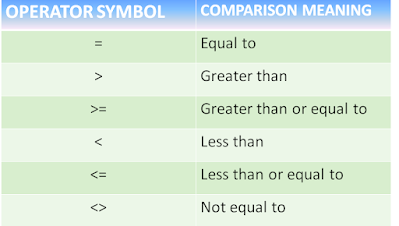
Logical or Comparison Operators
Logical operators are used to compare one value to another. They are called logical operators because the resultant answer is either FALSE or TRUE e.g 4>5 the answer is FALSE and 4<5 the answer is TRUE. When any of the comparisons operators are used in mathematical expressions excel can give only one of the two answers: TRUE or FALSE


Post a Comment